여름 휴가를 맞이하여 맹글고 있는 시난주 스타인~

이제 먹선작업까지 했습니다.... 그런데 ... 데칼 및 무광작업도 해야 하는데 힘드네요.... 

그래도, 여기까지 나름 잘 만들어진듯 합니다. 

시난주 스타인이 볼륨이 있어서인지 만드는 손맛도 있고 밸런스도 잘 맞아 좋은 기체인 듯 합니다.  ㅎㅎ

Understanding how SQL Server stores data in data files

By: Manvendra Singh   |   Read Comments   |   Related Tips: More > Database Administration

출처 : https://www.mssqltips.com/sqlservertip/4345/understanding-how-sql-server-stores-data-in-data-files/

Problem

Have you ever thought about how SQL Server stores data in its data files? As you know, data in tables is stored in row and column format at the logical level, but physically it stores data in data pages which are allocated from the data files of the database. In this tip I will show how pages are allocated to data files and what happens when there are multiple data files for a SQL Server database. 

Solution

Every SQL Server database has at least two operating system files: a data file and a log file. Data files can be of two types: Primary or Secondary.  The Primary data file contains startup information for the database and points to other files in the database. User data and objects can be stored in this file and every database has one primary data file. Secondary data files are optional and can be used to spread data across multiple files/disks by putting each file on a different disk drive. SQL Server databases can have multiple data and log files, but only one primary data file. Above these operating system files, there are Filegroups. Filegroups work as a logical container for the data files and a filegroup can have multiple data files.

The disk space allocated to a data file is logically divided into pages which is the fundamental unit of data storage in SQL Server. A database page is an 8 KB chunk of data. When you insert any data into a SQL Server database, it saves the data to a series of 8 KB pages inside the data file. If multiple data files exist within a filegroup, SQL Server allocates pages to all data files based on a round-robin mechanism. So if we insert data into a table, SQL Server allocates pages first to data file 1, then allocates to data file 2, and so on, then back to data file 1 again. SQL Server achieves this by an algorithm known as Proportional Fill.

The proportional fill algorithm is used when allocating pages, so all data files allocate space around the same time. This algorithm determines the amount of information that should be written to each of the data files in a multi-file filegroup based on the proportion of free space within each file, which allows the files to become full at approximately the same time. Proportional fill works based on the free space within a file.

Analyzing How SQL Server Data is Stored

Step 1: First we will create a database named "Manvendra" with three data files (1 primary and 2 secondary data files) and one log file by running the below T-SQL code. You can change the name of the database, file path, file names, size and file growth according to your needs.

CREATE DATABASE [Manvendra]
 CONTAINMENT = NONE
 ON  PRIMARY
( NAME = N'Manvendra', FILENAME = N'C:\MSSQL\DATA\Manvendra.mdf',SIZE = 5MB , MAXSIZE = UNLIMITED, FILEGROWTH = 10MB ),
( NAME = N'Manvendra_1', FILENAME = N'C:\MSSQL\DATA\Manvendra_1.ndf',SIZE = 5MB , MAXSIZE = UNLIMITED, FILEGROWTH = 10MB ),
( NAME = N'Manvendra_2', FILENAME = N'C:\MSSQL\DATA\Manvendra_2.ndf' ,SIZE = 5MB , MAXSIZE = UNLIMITED, FILEGROWTH = 10MB )
 LOG ON
( NAME = N'Manvendra_log', FILENAME = N'C:\MSSQL\DATA\Manvendra_log.ldf',SIZE = 10MB , MAXSIZE = 1GB , FILEGROWTH = 10%)
GO

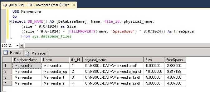
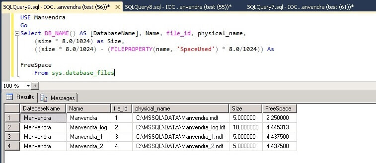
Step 2: Now we can check the available free space in each data file of this database to track the sequence of page allocations to the data files. There are multiple ways to check such information and below is one option. Run the below command to check free space in each data file.

USE Manvendra
GO
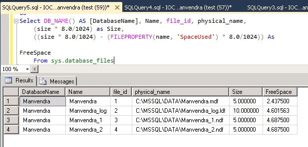
Select DB_NAME() AS [DatabaseName], Name, file_id, physical_name,
    (size * 8.0/1024) as Size,
    ((size * 8.0/1024) - (FILEPROPERTY(name, 'SpaceUsed') * 8.0/1024)) As FreeSpace
    From sys.database_files

You can see the data file names, file IDs, physical name, total size and available free space in each of the database files.

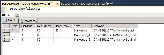
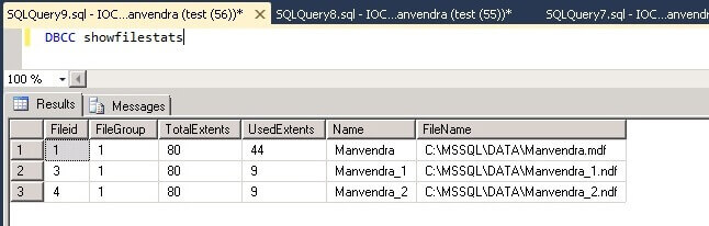
We can also check how many Extents are allocated for this database. We will run the below DBCC command to get this information. Although this is undocumented DBCC command this can be very useful information.

USE Manvendra
GO
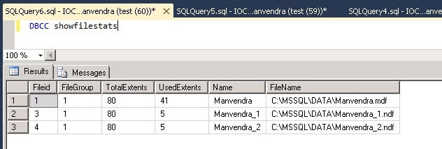
DBCC showfilestats

With this command we can see the number of Extents for each data file. As you may know, the size of each data page is 8KB and eight continuous pages equals one extent, so the size of an extent would be approximately 64KB. We created each data file with a size of 5 MB, so the total number of available extents would be 80 which is shown in column TotalExtents, we can get this by (5*1024)/64.

UsedExtents is the number of extents allocated with data. As I mentioned above, the primary data file includes system information about the database, so this is why this file has a higher number of UsedExtents.

Step 3: The next step is to create a table in which we will insert data. Run the below command to create a table. Once the table is created we will run both commands again which we ran in step 2 to get the details of free space and used/allocated extents.

USE Manvendra;
GO
CREATE TABLE [Test_Data] (
    [Sr.No] INT IDENTITY,
    [Date] DATETIME DEFAULT GETDATE (),
    [City] CHAR (25) DEFAULT 'Bangalore',
 [Name] CHAR (25) DEFAULT 'Manvendra Deo Singh');

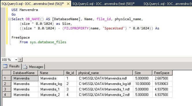
Step 4: Check the allocated pages and free space available in each data file by running same commands from step 2. 

USE Manvendra
Go
Select DB_NAME() AS [DatabaseName], Name, file_id, physical_name,
    (size * 8.0/1024) as Size,
    ((size * 8.0/1024) - (FILEPROPERTY(name, 'SpaceUsed') * 8.0/1024)) As FreeSpace
    From sys.database_files

You can see that there is no difference between this screenshot and the above screenshot except for a little difference in the FreeSpace for the transaction log file.

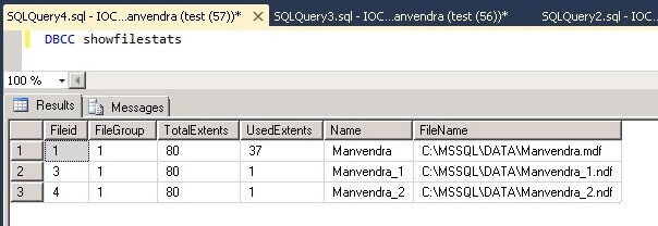
Now run the below DBCC command to check the allocated pages for each data file.

DBCC showfilestats

You can see the allocated pages of each data files has not changed.

Step 5: Now we will insert some data into this table to fill each of the data files. Run the below command to insert 10,000 rows to table Test_Data.

USE Manvendra
go
INSERT INTO Test_DATA DEFAULT VALUES;
GO 10000

Step 6: Once data is inserted we will check the available free space in each data file and the total allocated pages of each data file.

USE Manvendra
Go
Select DB_NAME() AS [DatabaseName], Name, file_id, physical_name,
    (size * 8.0/1024) as Size,
    ((size * 8.0/1024) - (FILEPROPERTY(name, 'SpaceUsed') * 8.0/1024)) As FreeSpace
    From sys.database_files

You can see the difference between the screenshot below and the above screenshot. Free space in each data file has been reduced and the same amount of space has been allocated from both of the secondary data files, because both files have the same amount of free space and proportional fill works based on the free space within a file. 

Now run below DBCC command to check the allocated pages for each data files.

DBCC showfilestats

You can see a few more pages have been allocated for each data file. Now the primary data file has 41 extents and the secondary data files have a total of 10 extents, so total data saved so far is 51 extents. Both secondary data files have the same number of extents allocated which proves the proportional fill algorithm.

Step 7: We can also see where data is stored for table "Test_Data" for each data file by running the below DBCC command. This will let us know that data is stored on all data files.

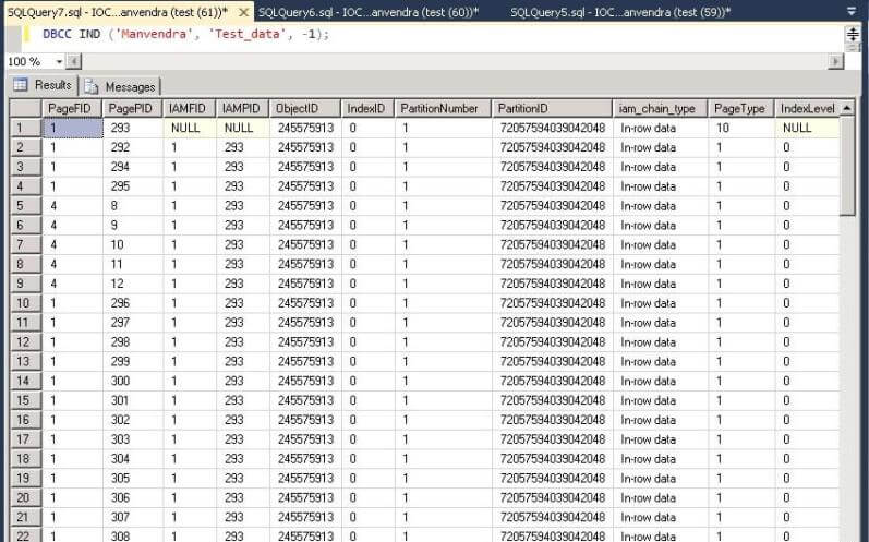
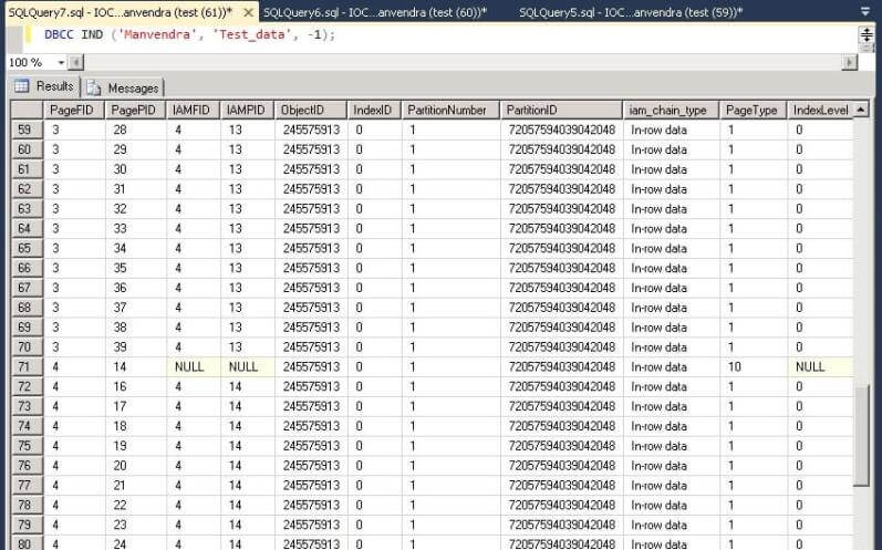
DBCC IND ('Manvendra', 'Test_data', -1);

I attached two screenshots because the number of rows was very large to show all data file IDs where data has been stored. File IDs are shown in each screenshot, so we can see each data page and their respective file ID. From this we can say that table Test_data is saved on all three data files as shown in the following screenshots.

Step 8: We will repeat the same exercise again to check space allocation for each data file. Insert an additional 10,000 rows to the same table Test_Data to check and validate the page allocation for each data file. Run the same command which we ran in step 5 to insert 10,000 more rows to the table test_data. Once the rows have been inserted, check the free space and allocated extents for each data file.

USE Manvendra
GO
INSERT INTO Test_DATA DEFAULT VALUES;
GO 10000
Select DB_NAME() AS [DatabaseName], Name, file_id, physical_name,
    (size * 8.0/1024) as Size,
    ((size * 8.0/1024) - (FILEPROPERTY(name, 'SpaceUsed') * 8.0/1024)) As FreeSpace
    From sys.database_files

We can see again both secondary data files have the same amount of free space and similar amount of space has been allocated from the primary data file as well. This means SQL Server uses a proportional fill algorithm to fill data in to the data files.

We can get the extent information again for the data files.

DBCC showfilestats

Again we can see in increase in the UsedExtents for all three of the data files.

Next Steps

• Create a test database and follow these steps, so you can better understand how SQL Server stores data at a physical and logical level. 
• Explore more knowledge with SQL Server Database Administration Tips

Graphing MySQL performance with Prometheus and Grafana

출처 : https://www.percona.com/blog/2016/02/29/graphing-mysql-performance-with-prometheus-and-grafana/